Tutorial: Stability of parallel shear flows

Background

Stability analysis of flows is a very important problem in fluid mechanics. Linearizing the Navier–Stokes equations around the mean flow and then eliminating pressure gives us the Orr–Sommerfeld and Squire equations, which are a system of fourth order PDEs describing the dynamics:

\[\left(\Big(\dfrac{\partial }{\partial t}+U\dfrac{\partial }{\partial x}\Big)\nabla^2-U''\dfrac{\partial }{\partial x}-\frac{1}{Re}\nabla^4\right)v = 0\\ \left(\dfrac{\partial }{\partial t}+U\dfrac{\partial }{\partial x}-\frac{1}{Re}\nabla^2\right)\eta = -U''\dfrac{\partial v}{\partial z}.\]

More precisely, these equations stem from modeling using a mean base laminar flow $\overline{U} = \begin{pmatrix}U(y)& 0& 0\end{pmatrix}$ and the perturbation $u' = \begin{pmatrix}u& v& w\end{pmatrix}$. The normal vorticity is denoted $\eta$.

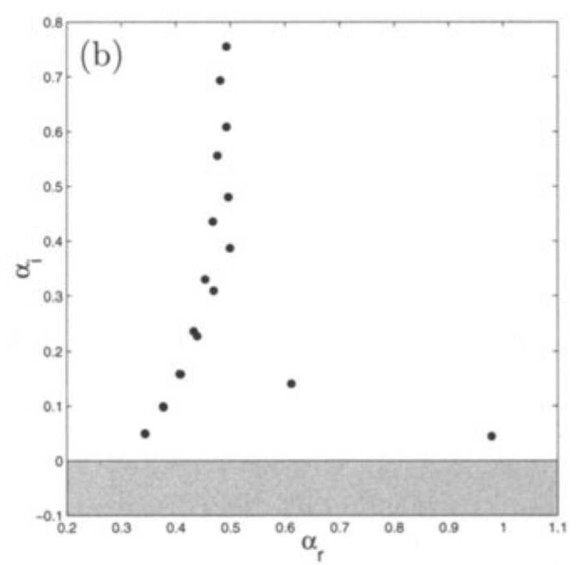
This is a text-book model for fluid flows. The model is often used to study stability by making a plane wave ansatz and a transformation, and subsequently rewriting the discretized problem as a large standard eigenvalue problem, see Chapter 7, Stability and Transition in Shear Flows, Schmid, Peter J., Henningson, Dan S. We will here show that the plane wave ansatz directly leads to a NEP, which can be solved with methods in NEP-PACK without any additional transformations. We reproduce computational results in the above reference.

We thank Miguel Beneitez and Prabal Negi, Department of Mechanics, KTH for the valuable discussions and the discretization code.

Formulation as a nonlinear eigenvalue problem

To study stability we use the plane wave perturbations ansatz

\[v(x,y,z,t) = \tilde{v}(y)\exp(i(\alpha x+\beta z-\omega t))\\ \eta(x,y,z,t) = \tilde{\eta}(y)\exp(i(\alpha x+\beta z-\omega t)),\]

which transforms the system to

\[\left((-i\omega+i\alpha U)(\mathcal{D}^2-\alpha^2-\beta^2)-i\alpha U''-\frac{1}{Re}(\mathcal{D}^2-\alpha^2-\beta^2)^2\right)\tilde{v} = 0,\\ \left((-i\omega+i\alpha U)-\frac{1}{Re}(\mathcal{D}^2-\alpha^2-\beta^2)\right)\eta = -i\beta U'\tilde{v},\]

where $\mathcal{D}$ denotes the 1-D differential operator $\frac{\partial }{\partial y}$. In this example, we consider the boundary conditions $\tilde{v} = \mathcal{D}\tilde{v} = \tilde{\eta} = 0$. We assume that $\beta$ and $\omega$ are given and we wish to solve for the eigenvalue $\alpha\in\mathbb{C}$.

This is usually done by using a transformation of the form

\[\begin{pmatrix}\tilde{v}\\ \tilde{\eta}\end{pmatrix} = \begin{pmatrix}\tilde{V}\\ \tilde{E}\end{pmatrix}\exp(-\alpha y)\]

which reduces the power of $\alpha$ from four to two. The problem is then discretized and solved as a quadratic eigenvalue problem. See Chapter 7 in Schmid–Henningson for details.

Rather than using the transformation approach described in the book of Schmid–Henningson, we simply discretize $\mathcal{D}$ to $D$ (using a suitable numerical discretization) which leads to a polynomial eigenvalue problem of fourth order.

We define diagonal matrices $U_0$, $U_1$ and $U_2$ as follows

\[U_0 = diag(U(y_0),U(y_1),\ldots,U(y_n)),\\ U_1 = diag(U'(y_0),U'(y_1),\ldots,U'(y_n)),\\ U_2 = diag(U''(y_0),U''(y_1),\ldots,U''(y_n)),\]

where $\{y_i\}_{i=1,\ldots,n}$ denotes the y-coordinates of the $n$ grid points used for discretization. The discretized problem, after expanding the powers, gives

\[\left[-\frac{I}{Re}\alpha^4-iU_0\alpha^3+\left(\frac{2D^2}{Re}+\left(i\omega- \frac{2\beta^2}{Re}\right)I\right)\alpha^2\right.+\\ \left.\left(iU_0(D^2-\beta^2I)-U_2\right)\alpha +\Big(\frac{2\beta^2D^2}{Re}-\frac{D^4}{Re}-\frac{\beta^4I}{Re}+i\omega(\beta^2I-D^2)\Big)\right]\tilde{v} = 0\\ i\beta U_1\tilde{v}+\left[\frac{I}{Re}\alpha^2 + iU_0 \alpha +\left(\left(\frac{\beta^2}{Re}-i\omega\right)I-\frac{D^2}{Re}\right)\right]\tilde{\eta} = 0.\]

This can be be formulated as a polynomial eigenvalue problem

\[M(\lambda) = A_0+A_1\lambda+A_2\lambda^2+A_3\lambda^3+A_4\lambda^4,\]

and the matrices $A_0,\ldots,A_4$ are given by

\[A_0 = \begin{pmatrix}\frac{2\beta^2D^2}{Re}-\frac{D^4}{Re}-\frac{\beta^4I}{Re}+i\omega(\beta^2I-D^2)& 0\\ i\beta U_1&\left(\frac{\beta^2}{Re}-i\omega\right)I-\frac{D^2}{Re}\end{pmatrix}\\ A_1 = \begin{pmatrix}iU_0(D^2-\beta^2I)-U_2& 0\\0& iU_0\end{pmatrix}\\ A_2 = \begin{pmatrix}\frac{2D^2}{Re}+\left(i\omega- \frac{2\beta^2}{Re}\right)I& 0\\0& \frac{I}{Re}\end{pmatrix}\\ A_3 = \begin{pmatrix}-iU_0& 0\\0& 0\end{pmatrix}\\ A_4 = \begin{pmatrix}-\frac{I}{Re}& 0\\0& 0\end{pmatrix}.\]

The eigenvector is given by $\begin{pmatrix}\tilde{v}^T & \tilde{\eta}\end{pmatrix}^T$

Problem setup in NEP-PACK

The tutorial uses the helper-functions chebdif and cheb4c, which are provided in cheb4c.jl and chebdif.jl.

using NonlinearEigenproblems, Plots, ToeplitzMatrices;
include("cheb4c.jl");
include("chebdif.jl");

We begin by initializing the parameters to the values used to generate the data in Table 7.1 in Schmid–Henningson.

N = 256;      # Number of interior points
Re = 2000;    # Reynolds number
ω  = 0.3;     # Input frequency
β  = 0.0;     # Spanwise wavenumber

To set up the matrices $A_i$, we need the discretized matrices corresponding to the operators $\mathcal{D}^2$ and $\mathcal{D}^4$. Here, we do this using Chebyshev nodes.

# Çhebyshev discretization of differential operators
yF,DM = chebdif(N+2, 4);    
D2 = DM[2:N+1,2:N+1,2];              #D^2
yF,D4 = cheb4c(N+2);                 #D^4

# The base flow for Poiseuille plane flow
U   = 1 .-yF.^2;
Up  = -2*yF;
Upp = -2;

eye = Matrix{Float64}(I, N, N);

We can now set up the coefficient matrices and create a corresponding PEP object.

A4 = [-eye/Re zeros(N,N);zeros(N,N) zeros(N,N)];
A3 = [-1im*diagm(0 => U) zeros(N,N);zeros(N,N) zeros(N,N)];
A2 = [(1im*ω-2β^2/Re)*eye+2D2/Re zeros(N,N);zeros(N,N) eye/Re];
A1 = [1im*(diagm(0 => U)*(D2-eye*β^2)-Upp*eye) zeros(N,N);zeros(N,N) 1im*diagm(0=>U)];
A0 = [2β^2*D2/Re-D4/Re-β^4*eye/Re+1im*ω*(β^2*eye-D2) zeros(N,N);1im*β*diagm(0 => Up) (-1im*ω+β^2/Re)*eye-D2/Re];
nep = PEP([A0,A1,A2,A3,A4]); #Create a PEP object

Solving with NEP-PACK

Because of poorly scaled coefficient matrices, direct application of NEP-PACK's solvers on this problem is inadequate. We note that the norm of the coefficient matrices are:

julia> norm.(get_Av(nep))
5-element Array{Float64,1}:
      8.37194982854379e13
 473949.06740743306      
 303285.4108872535       
      9.817076958035932  
      0.008

Fortunally we can get around this issue by scaling the PEP with NEP-PACK's shift_and_scale , and solving the scaled problem $T(\lambda) = M(100\lambda)$ instead.

sc=100;
nep1 = shift_and_scale(nep,scale=sc);
mult_scale = norm(nep1.A[end]);
nep2 = PEP(nep1.A ./ mult_scale);

The scaled PEP has much better scaled coefficient matrices.

julia> norm.(get_Av(nep2))
5-element Array{Float64,1}:
    1.0464937285679738e8
   59.24363342592913    
 3791.0676360906696     
   12.271346197544913   
    1.0

In this example, we are interested in computing several eigenvalues and our region of interest for the spectrum is in the first quadrant. We use the Tensor Infinite Arnoldi (TIAR) method implemented in tiar. The method is called twice with different shifts σ.

λ1,v1 = tiar(nep2,σ=0.006,v=ones(size(nep,1)),neigs=10,maxit=200,tol=1e-14);
λ2,v2 = tiar(nep2,σ=0.005+0.005im,v=ones(size(nep,1)),neigs=10,maxit=200,tol=1e-14);
λtotal = [λ1;λ2];

The computed eigenvalues are scaled back to get the eigenvalues of the original problem.

 julia> λ_orig = sc*λtotal
20-element Array{Complex{Float64},1}:
  0.3765784040323032 + 0.09959915134763689im
 0.30865495875240445 + 0.008960297181538185im
  0.4087137042139992 + 0.15906877547743775im
  0.9787481874161135 + 0.0443939782417711im  
  0.3430534698620533 + 0.049837687199345705im
 -0.2863097014631293 - 0.9011417554715162im  
  0.6116671743160434 + 0.14049254864376023im
 0.40933722321954447 + 0.15820580776369225im
 0.43950860634751715 + 0.22808195062035772im
 0.37687009160849716 + 0.09924325053688597im
 0.47944942696208637 + 0.40059913080096726im
  0.4934801111510124 + 0.520295324777746im   
   0.496596553706975 + 0.480303769976205im   
 0.49307795048742775 + 0.6085434637464817im  
  0.5095613980300516 + 0.6639488620533516im  
  0.4998069928360967 + 0.3870365082453997im  
  0.4861657916302239 + 0.45751028495939855im
  0.4766598864386299 + 0.5557787925858408im  
  0.4684227095574837 + 0.4353215518427161im  
  0.5014319544500476 + 0.5889845608687214im

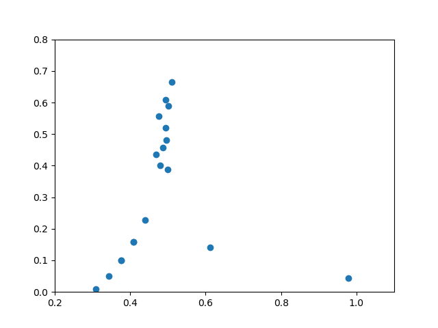
The computed eigenvalues in the first quadrant can be plotted by:

julia> plot(real.(λ_orig),imag.(λ_orig),seriestype=:scatter,xaxis=[0.2,1.05],yaxis=[0,0.8])

The resulting plot is:

This is in agreement with Figure 7.2 from Schmid–Henningson for the eigenvalues in the first quadrant.