Tutorial: User-defined matrices - boundary element method

Suppose you have a new type of NEP, which does not naturally fit into the standard types in NEP-PACK. This tutorial shows how you can define a NEP where the only way to access the NEP is a function to compute $M^{(k)}(λ)$. We first show the manual way to do it, as it illustrates some of the workings of NEP-PACK. However, the use case is common enough to have native support in NEP-PACK. Hence, we also show how to use a special NEP-type called Mder_NEP.

For this example we use a boundary element method approach for computation of resonances. The complete code is available in gallery_extra/bem_hardcoded. The example is also available as a gallery problem: nep=nep_gallery("bem_fichera").

Boundary element method

The boundary element method applied to Helmholtz eigenvalue problem can be described by the matrix consisting of elements

where $\Delta_i$, $i=1,\ldots,n$ are boundary elements. The boundary element approach is available through three functions: gen_ficheramesh to compute the mesh, precompute_quad! to precompute the quadrature coeeficients, and assemble_BEM to compute the matrix consisting of all the integrals corresponding to λ. These functions are based on the model (and inspired by some of the code) in "A boundary element method for solving PDE eigenvalue problems", Steinlechner, bachelor thesis, ETH Zürich, 2010 and also used in the simulations in "Chebyshev interpolation for nonlinear eigenvalue problems", Effenberger, Kressner, BIT Numerical Mathematics, 2012, Volume 52, Issue 4, pp 933–951.

To get access to the helper functions you need either to work in the gallery_extra/bem_hardcoded-directory, or copy the files in there to your current working directory. The code can also be found directly on github. We start by loading the necessary code:

julia> using NonlinearEigenproblems;
julia> include("triangle.jl");
julia> include("genmesh.jl");
julia> include("assemble_BEM.jl");

Manual implementation in NEP-PACK

In order to define your new NEP you need to define a new NEP-type

julia> struct BEM_NEP <: NEP
    mesh::Vector{Triangle}
    n::Int
    gauss_order::Int
    function BEM_NEP(mesh,gauss_order)
        return new(mesh,length(mesh),gauss_order)
    end
end

The mesh variable is a vector of triangle objects defining the domain, n is the size of the mesh and gauss_order the quadrature order. All NEPs have to define size() functions

julia> import Base.size; # Import from Base explicitly since we overload

julia> function size(nep::BEM_NEP)
    return (nep.n,nep.n);
end
size (generic function with 142 methods)
julia> function size(nep::BEM_NEP,dim)
    return nep.n;
end
size (generic function with 143 methods)

The function assemble_BEM computes the matrix defined by the integrals. Hence, we need to call this function for every call to compute_Mder:

julia> import NonlinearEigenproblems.NEPCore.compute_Mder # We overload the function
julia> function compute_Mder(nep::BEM_NEP,λ::Number,der::Int=0)
    return assemble_BEM(λ, nep.mesh, nep.gauss_order, der)[:,:,1];
end
compute_Mder (generic function with 42 methods)

In order to make other compute functions available to the methods, we can use the conversion functions. In particular, the compute_Mlincomb function can be implemented by making several calls in compute_Mder. This is done in the NEP-PACK-provided helper function compute_Mlincomb_from_Mder. We make this the default behaviour for this NEP:

julia> import NonlinearEigenproblems.NEPCore.compute_Mlincomb # Since we overload
# Delegate the compute Mlincomb functions. This can be quite inefficient.
julia> compute_Mlincomb(nep::BEM_NEP,λ::Number,V::AbstractVecOrMat, a::Vector) =
      compute_Mlincomb_from_Mder(nep,λ,V,a)
compute_Mlincomb (generic function with 36 methods)
julia> compute_Mlincomb(nep::BEM_NEP,λ::Number,V::AbstractVecOrMat) =
      compute_Mlincomb(nep,λ,V, ones(eltype(V),size(V,2)))
compute_Mlincomb (generic function with 37 methods)

We can now create a BEM_NEP as follows:

julia> gauss_order=3; N=5;
julia> mymesh=gen_ficheramesh(N);
julia> precompute_quad!(mymesh,gauss_order);
julia> nep=BEM_NEP(mymesh,gauss_order);

Solving the NEP

After creating the NEP, you can try to solve the problem with methods in the package, e.g., mslp works quite well for this problem:

julia> (λ,v)=mslp(nep,λ=8,logger=1);
iter 1 err:4.122635537095191e-6 λ=8.128272919317748 + 0.007584851218213724im
iter 2 err:1.787963303966838e-8 λ=8.132181234599429 - 1.952792817333862e-5im
iter 3 err:3.2884911876526185e-13 λ=8.132145310156645 - 1.2648247030082216e-5im
iter 4 err:4.417989064002117e-18 λ=8.132145310195458 - 1.264891803723658e-5im

This is the computed solution:

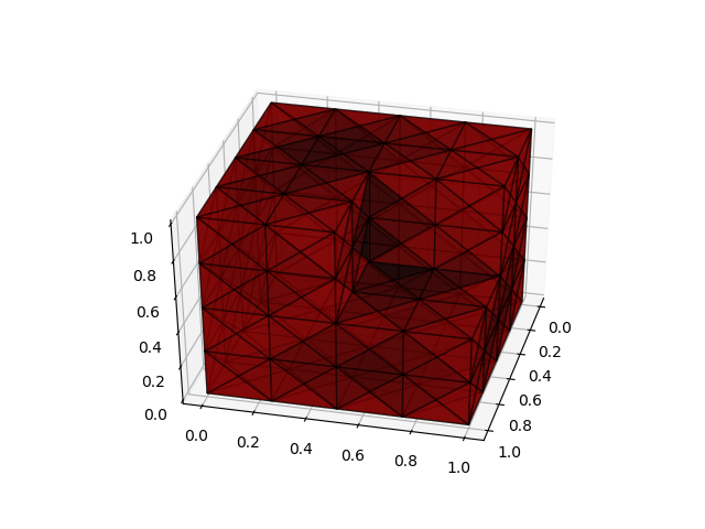
The plotting was done with the following code (by using internals of the BEM-implementation):

julia> using PyPlot
julia> v=v./maximum(abs.(v));
julia> for k=1:size(nep.mesh,1);
    tri=nep.mesh[k];
    col=[1-abs.(v)[k];0;0]; # plot abslolute value
    X=[tri.P1[1] tri.P2[1]; tri.P3[1] tri.P3[1]];
    Y=[tri.P1[2] tri.P2[2]; tri.P3[2] tri.P3[2]];
    Z=[tri.P1[3] tri.P2[3]; tri.P3[3] tri.P3[3]];
    plot_surface(X,Y,Z,color=col,alpha=0.8);
    plot_wireframe(X,Y,Z,color=[0;0;0],linewidth=1,alpha=0.5,);
end

Implementation in NEP-PACK using the Mder_NEP type

Some of the manual implementation can be avoided by using the Mder_NEP type. We only need to pass the size of the NEP and a function to compute $M^{(k)}(λ)$, i.e., (λf,derf) -> assemble_BEM(λf, mymesh, gauss_order, derf)[:,:,1], to the Mder_NEP.

julia> n = length(mymesh);
julia> mdernep = Mder_NEP(n, (λf,derf) -> assemble_BEM(λf, mymesh, gauss_order, derf)[:,:,1]);
julia> (mderλ,mderv)=mslp(mdernep,λ=8,logger=1);
iter 1 err:4.122635537095191e-6 λ=8.128272919317748 + 0.007584851218213724im
iter 2 err:1.787963303966838e-8 λ=8.132181234599429 - 1.952792817333862e-5im
iter 3 err:3.2884911876526185e-13 λ=8.132145310156645 - 1.2648247030082216e-5im
iter 4 err:4.417989064002117e-18 λ=8.132145310195458 - 1.264891803723658e-5im
julia> λ-mderλ
0.0 + 0.0im

precompute_quad!(mymesh,gauss_order);