Tutorial: Application to absorbing boundary conditions

A Schrödinger equation

We consider the Schrödinger type eigenvalue problem on the interval $[0,L_1]$,

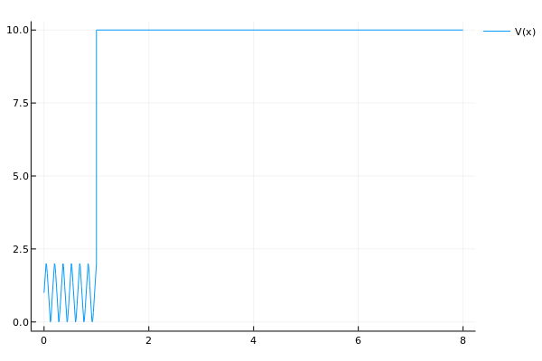
\[\begin{eqnarray*} \left( \frac{\partial^2}{\partial x^2} -V(x)-\lambda \right)\psi(x)&=&0,\,\; x\in[0,L_1]\\ \psi(0)&=&0\\ \psi(L_1)&=&0. \end{eqnarray*}\]

We wish to compute eigenvalue $λ$ and eigenfunction $\psi$. Moreover, we assume that the potential function $V(x)$ is benign in the domain $[L_0,L_1]$, in our case for simplicity it is constant, such that we can later solve the problem in that domain analytically. In the simulations we will consider this function

\[ V(x)= \begin{cases} 1+\sin(\alpha x) & x\in[0,L_0]=[0,1]\\ V_0 & x\in(L_0,L_1)=(1,8) \end{cases}\]

where $α$ is large, i.e., the potential has high frequency oscillations in one part of the domain.

This tutorial illustrates how we can avoid a discretization of the domain $[L_0,L_1]$ and only discretize $[0,L_0]$, by solving a NEP. The implementation described below is also directly available in the gallery: nep_gallery("schrodinger_movebc").

Derivation of reduced domain differential equation

The technique is based on moving the boundary condition at $L_1$ to $L_0$. This can be done without doing any approximation, if we allow the new artificial boundary condition at $L_0$ to depend on $λ$. We introduce what is called an absorbing boundary condition, also known as an artificial boundary condition.

We first note that we can transform the problem to first order form

\[ \frac{d}{dx} \begin{bmatrix}\psi(x)\\\psi'(x)\end{bmatrix} = \begin{bmatrix} 0 & 1\\ \lambda+V(x) & 0 \end{bmatrix} \begin{bmatrix}\psi(x)\\\psi'(x)\end{bmatrix}.\]

The potential $V(x)$ is constant in the domain $[L_0,L_1]$. This allows us to directly express the solution using the matrix exponential

\[\begin{bmatrix}\psi(x)\\\psi'(x)\end{bmatrix} =\exp\left((x-L_0) \begin{bmatrix} 0 & 1\\ \lambda+V_0 & 0 \end{bmatrix} \right) \begin{bmatrix}\psi(L_0)\\\psi'(L_0)\end{bmatrix}.\]

when $x\in[L_0,L_1]$. The boundary condition $\psi(L_1)=0$ can be imposed as

\[0=\psi(L_1)=\begin{bmatrix}1 & 0\end{bmatrix} \begin{bmatrix}\psi(L_1)\\\psi'(L_1)\end{bmatrix} =\begin{bmatrix}1 & 0\end{bmatrix}\exp\left((L_1-L_0) \begin{bmatrix} 0 & 1\\ \lambda+V_0 & 0 \end{bmatrix} \right) \begin{bmatrix}\psi(L_0)\\\psi'(L_0)\end{bmatrix}.\]

By explicitly using the hyperbolic functions formula for the matrix exponential of an antidiagonal two-by-two matrix we obtain the relation

\[0= g(λ)\psi(L_0)+ f(λ)\psi'(L_0).\]

where

\[g(λ):=\cosh\left((L_1-L_0)\sqrt{λ+V_0}\right)\]

\[f(λ):=\frac{\sinh\left((L_1-L_0)\sqrt{λ+V_0}\right)}{\sqrt{λ+V_0}}.\]

Note that a solution to the original boundary value problem will satisfy the condition $0=g(λ)\psi(L_0)+f(λ)\psi'(L_0)$, which involves only the point $x=L_0$, i.e., the middle of the domain. We can now disconnect the problem and only consider only the domain $[0,L_0]$ by using this condition instead, since a solution to the original boundary value problem satisfies

\[\begin{eqnarray*} \left( \frac{\partial^2}{\partial x^2} -V(x)-\lambda \right)\psi(x)&=&0,\,\; x\in[0,L_0]\\ \psi(0)&=&0\\ g(λ)\psi(L_0)+f(λ)\psi'(L_0)&=&0. \end{eqnarray*}\]

which is a boundary value problem on the reduced domain $[0,L_0]$. The boundary condition is a Robin boundary condition (also called mixed boundary condition) at $x=L_0$, since it contains both $\psi(L_0)$ and $\psi'(L_0)$. It can be shown that the solutions to the original problem are the same as the solutions on the reduced domain, except for some unintresting special cases.

Discretization of the λ-dependent boundary value problem

The boundary condition in the reduced domain boundary value problem is λ-dependent. Therefore a standard discretization the domain $[0,L_0]$, e.g., finite difference, will lead to a nonlinear eigenvalue problem. More precisely, we discretize the problem as follows.

Let $x_k=hk$, $k=1,\ldots n$ and $h=1/n$ such that $x_1=h$ and $x_n=1=L_0$. An approximation of the $\lambda$-dependent boundary condition can be found with the one-sided second order difference scheme

\[ 0=g(λ)\psi(L_0)+f(λ)\frac{1}{h}\left(\frac32 \psi(L_0) -2\psi(x_{n-1}) +\frac12\psi(x_{n-2})\right)+O(h^2).\]

Let

\[ D_n= \frac1{h^2} \begin{bmatrix} -2 & 1 & 0 &\\ 1 & \ddots &1& \\ 0 & 1 &-2 & 1\\ 0 & \cdots & 0 & 0 \end{bmatrix}\;\textrm{ and }\; \underline{I}_n=\begin{bmatrix}1 &\\ &\ddots\\ &&1 \\ & &&0\end{bmatrix}\]

Then the boundary value problem can expressed as

\[M(λ)v=0\]

where

\[M(λ)=A-λ\underline{I}_n +g(λ)e_ne_n^T+f(λ)F,\]

and

\[A=D_n-\operatorname{diag}(V(x_1),\ldots,V(x_{n-1}),0),\;\;F=\frac{1}{2h}e_ne_{n-2}^T-\frac{2}{h}e_ne_{n-1}^T+\frac{3}{2h}e_ne_n^T.\]

Implementation in NEP-PACK

The above discretization can be expressed as a SPMF_NEP with four terms. Let us set up the matrices first

using LinearAlgebra,SparseArrays;
L0=1; L1=8; V0=10.0;
xv=Vector(range(0,stop=L0,length=1000))
h=xv[2]-xv[1];
n=size(xv,1);
α=25*pi/2;
V=x->1+sin(α*x);
Dn=spdiagm(-1 => [ones(n-2);0]/h^2, 0 => -2*ones(n-1)/h^2, 1 => ones(n-1)/h^2)
Vn=spdiagm(0 => [V.(xv[1:end-1]);0]);
A=Dn-Vn;
In=spdiagm(0 => [ones(n-1);0])
F=sparse([n, n, n],[n-2, n-1, n],[1/(2*h), -2/h, 3/(2*h)])
G=sparse([n],[n],[1]);

The corresponding functions in the SPMF are defined as follows

f1=S->one(S);
f2=S->-S;
hh=S-> sqrt(S+V0*one(S))
g=S-> cosh((L1-L0)*hh(S))
f=S-> inv(hh(S))*sinh((L1-L0)*hh(S))

Note that when defining an SPMF, all functions should be defined in a matrix function sense (not element-wise sence). Fortunately, in Julia, sinh(A) and cosh(A) for matrix A are interpreted as matrix functions. The NEP can now be created and solved by directly invoking the SPMF-creator and applying a NEP-solver:

using NonlinearEigenproblems
nep=SPMF_NEP([Dn-Vn,In,G,F],[f1,f2,g,f]);
(λ1,v1)=quasinewton(Float64,nep,logger=1,λ=-5,v=ones(n),tol=1e-9);
(λ2,v2)=quasinewton(nep,logger=1,λ=-11,v=ones(n),tol=1e-9)
(λ3,v3)=quasinewton(nep,logger=1,λ=-20,v=ones(n),tol=1e-9)
(λ4,v4)=quasinewton(nep,logger=1,λ=-35,v=ones(n),tol=1e-9)

We can easily do a sanity check of the solution by visualizing it in this way

using Plots
plot(xv,v1/norm(v1))
plot!(xv,real(v2)/norm(v2))
plot!(xv,real(v3)/norm(v3))
plot!(xv,real(v4)/norm(v4))

resulting in

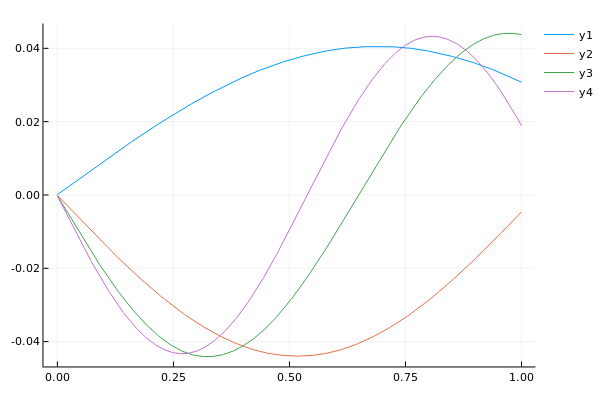
Rather than making several calls to a specific method, some NEP-solvers directly compute several solutions. The NEP-solver iar works quite well for this problem (see also the deflation approach to compute several solutions):

julia> (λ,v)=iar(nep,logger=1,σ=-36,v=ones(n),tol=1e-9,neigs=5,maxit=100);
-
--
---
----
-----
------
=------
+-------
+--------
+---------
+----------
+-----------
+=-----------
++------------
++-------------
++--------------
++---------------
++----------------
+++----------------
++=-----------------
++=------------------
+++-------------------
+++--------------------
+++---------------------
+++----------------------
+++-----------------------
+++------------------------
+++-------------------------
+++=-------------------------
+++=--------------------------
++++---------------------------
++++----------------------------
++++-----------------------------
++++------------------------------
++++-------------------------------
++++--------------------------------
++++=--------------------------------
+++++---------------------------------
julia> λ
5-element Array{Complex{Float64},1}:
  -34.93072323018405 + 4.272712516424266e-18im
  -39.14039540604307 + 2.054980381709175e-16im
 -31.057106551809486 - 3.2616991503097867e-15im
  -43.66198303378091 - 4.3753274496659e-15im
 -27.537645678335437 + 4.8158177866759774e-15im

The output of the logging of iar is a compact notation for how many eigenvalues have converged at a specific iteration. Every line corresponds to one iteration step. The signs correspond to: +=a converged eigenvalue, -=not converged eigenvalue, ==almost converged eigenvalue in the sense that it almost (up to a factor 10) satisfies the convergence criteria.

Tip

The performance of many NEP-algorithms for this problem can be improved. One improvement is achieved with a simple variable transformation. If we let $\mu=\sqrt{\lambda+V_0}$ we have $\lambda=\mu^2-V_0$. Therefore the NEP can be transformed in a way that it does not contain square roots. Square roots are undesirable, since they can limit convergence in many methods due to the fact that they are not entire functions. The $\sinh$ and $\cosh$ can be merged to a $\tanh$-expression, leading to less nonlinear terms (but possibly more difficult singularities).

Verifying the solution

Let us verify the solution with a direct discretization of the domain. The ApproxFun.jl package provides tools to solve differential equations in one dimension. We use this package to discretize the entire domain $[0,L_1]$, whereas only a discretization of $[0,L_0]$ is necessary in the NEP-approach.

The eigenvalues of the operator can be computed as follows (where we approximate the singular point of the potential with a regularized heaviside function).

julia> using LinearAlgebra, ApproxFun;
julia> x = Fun(0 .. 8)
julia> V0 = 10;
julia> α = 25*pi/2;
julia> # Let Ha be an approximation of H(x-1) where H is a Heaviside function
julia> kk=10; Ha = 1 ./(1+exp(-2*kk*(x .- 1.0)));
julia> VV=V0*Ha + (1-Ha) * sin(α*x)
julia> L = 𝒟^2-VV
julia> S = space(x)
julia> B = Dirichlet(S)
julia> ee= eigvals(B, L, 500,tolerance=1E-10);

We obtain approximations of the same eigenvalues as with the NEP-approach

julia> ee[sortperm(abs.(ee.+36))[1:5]]
 -34.85722089717211
 -39.051578662445074
 -30.984470654329677
 -43.54933251507695
 -27.450712883781343

To the top